Generate Bayesian Network
Clicking Create Bayesian Network after you have configured the settings on the Bayesian Network screen navigates you to the generated model screen.
All the available network Views are shown in a series of tabs. The following actions are available at the top right of the tab bar:
- Algorithm Settings: Allows you to re-configure the algorithms used to generate the model
- New Bayesian Network: Restarts the generation process
-
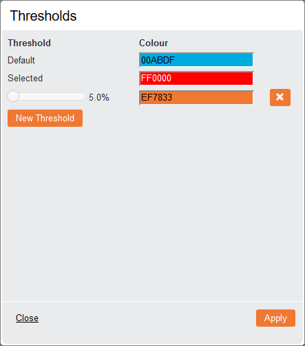
Conditional Formatting (applies only to Tile View and Model views): Allows you to customise the colours used when thresholds are met. This will change the colour of the outcome bars that have changed by more than the threshold percentage.

Click New Threshold to create an entry, then use the slider to select a desired percentage. Then choose a colour either by typing in the hex code or using the pop-up colour selector. When all thresholds are set, click Apply to save the changes.
- Redraw Network: Resets the layout
Display Options
The following options are used across the view tabs:
| Option(s) | View(s) it applies to | Description |
|---|---|---|
| Add Field | Summary, Tile View, Model, Visualisations |
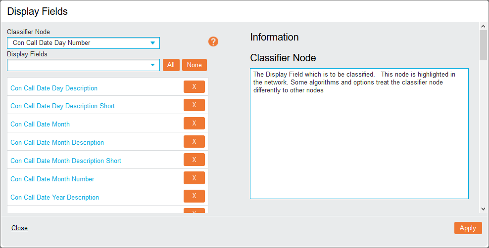
Allows you to change the fields that are used in the network.
Select the Classifier Node and select the Display Fields used in the network from the drop-down lists. Fields can also be removed using the x icon next to the field name. Click Apply to apply your changes and close the window. |
| Show All | Summary, Tile View, Model. Visualisations | Displays all fields originally specified before the generation process. |
| Hide Disconnected | Summary, Tile View, Model, Visualisations | Hides any fields in the network that have not been conditionally linked. |
| Sort | Tile View, Model, Visualisations |
Sorts the nodes by one of the following methods:
|
|
(Lock Node Zoom) |
Model | Toggles the automatic zooming when the cursor moves over a node in the network. Changes to the ‘lock’ position when selected. |
|
(Dynamic Line Thickness) |
Model | Toggles how the dependency arrows are displayed. With the option enabled, arrows will vary in thickness depending on how much of an effect probability manipulation will affect the connected node. The thicker the arrow, the higher the dependency. Changes to the thick arrow once selected. |
Outcome Options
The following options are available for each displayed field in Summary, Tile View and Model tabs:
| Icon | Option | Description |
|---|---|---|
|
|
Hide Field | Hides the field from the network. Hidden fields are displayed at the bottom of the list under the Hidden title. |
|
|
Show Hidden Field | Restores a hidden field to the network and moves the field to the original location in the list. |
|
|
Field Options |
Displays the following options:
|
|
|
Select Outcome |
Allows you to manipulate the probability of an individual field to simulate controlled probabilities. Click either Select Outcome or the value in the 'Most Likely Outcome' column of a field and select a value. This will change the probability of this event to 100%, allowing the evaluation of an individual belief on the rest of the network. The rest of the network will automatically update as probabilities are manipulated, with percentage changes highlighted next to each individual probability. There is no limit to how many nodes can be manipulated, allowing predictions to be made when specific circumstances are met. The current selections are shown under the navigation tabs and can be cleared fully by clicking the x icon next to All Current Selections or individually by clicking the x icon next to the field name. As with all statistical models, accuracy is reliant on the quality of the data analysed and algorithms used. |
|
|
Remove Field | Removes the field from the network. This will display a dialog box, click OK to rerun the network without the selected field. The classifier node cannot be removed. |
Views
You can access the views through the following tabs:
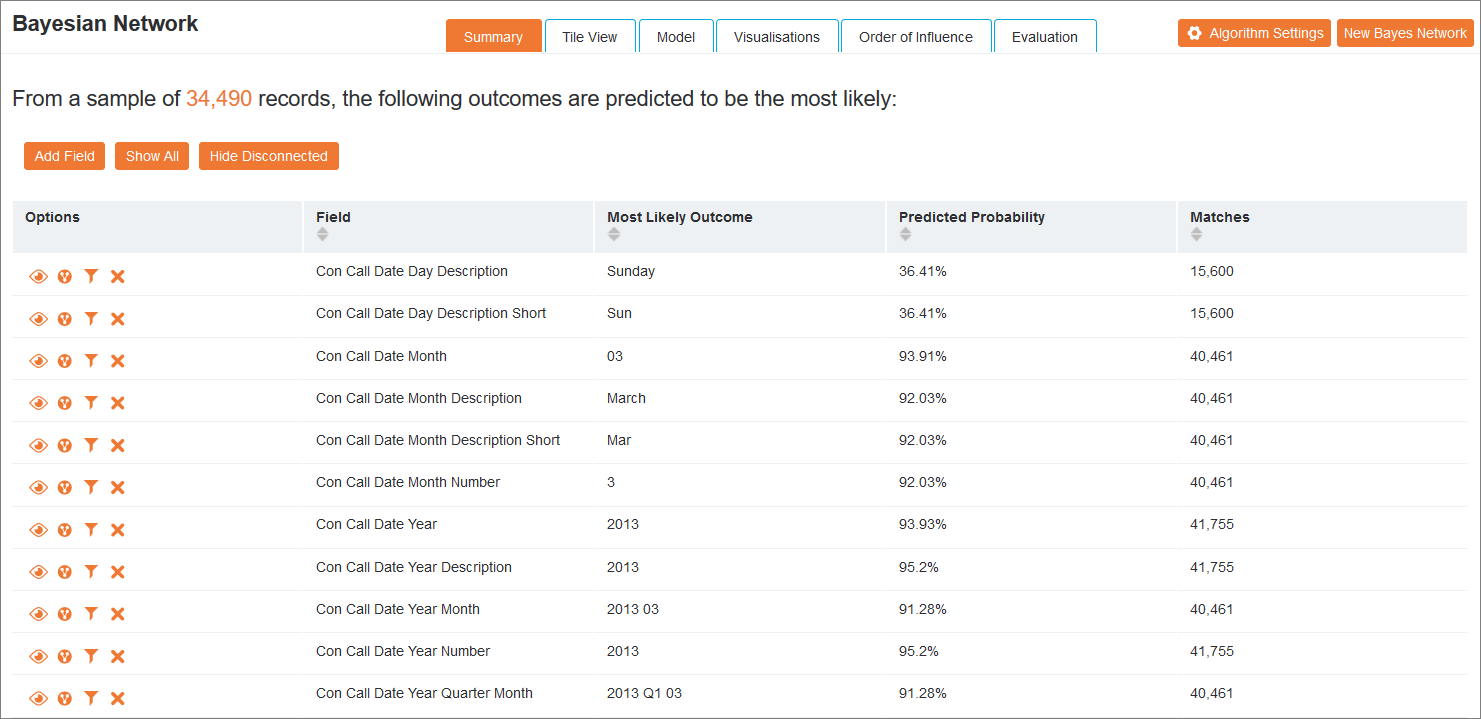
The Summary view shows a list with the outcomes that are predicted to be the most likely once a network has been generated. In the displayed table each field is listed with the outcome deemed most likely, predicted probability and the number of matches in the network.
If one or more probabilities has been manipulated, the Change from Original Probability column will be automatically displayed to reflect the changes made to connected fields. The individual fields that have been modified are shown at the top of the page.
On the left of each row there are the Outcome Options.
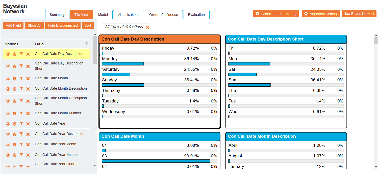
This view presents all nodes in a network in rows for fast navigation. The navigation pane on the left of the screen lists all currently included fields with their Outcome Options. As the cursor moves over a node, the corresponding field is highlighted in this list.
Tip: This view is especially useful when viewing a large network.
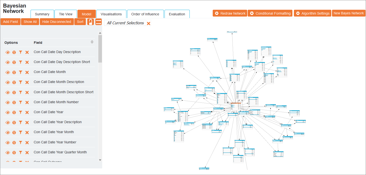
This view displays the nodes and arrows representing their conditional dependencies as a directed acyclic graph (DAG). By default, the classifier node is orange and the other nodes are blue.
Nodes can be repositioned on the screen by dragging and dropping them and will automatically zoom when the cursor moves over them. To disable zooming, click the lock ![]() icon in the Display Options. To reset the layout, click Redraw Network at the top of the screen.
icon in the Display Options. To reset the layout, click Redraw Network at the top of the screen.
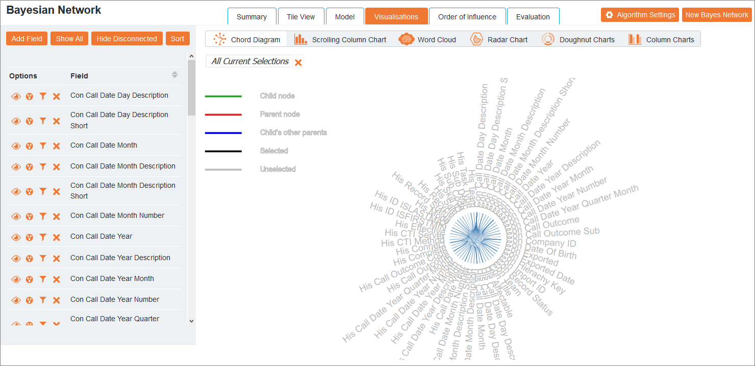
The Visualisations view presents the network in a number of ways:
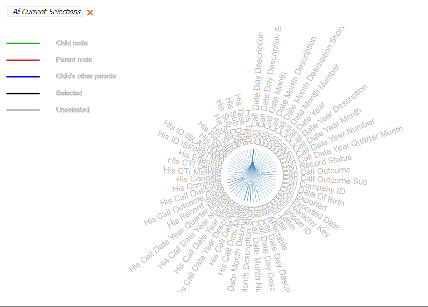
Moving the cursor over a field name reveals the connected fields and whether it is a child node, parent node, child’s other parent, selected or unselected. This diagram is useful for quickly discovering the fields that have a direct connection in the network.
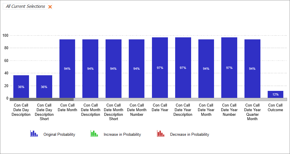
Displays fields and their current probabilities. When the nodes are manipulated, the percentage change to each probability will be displayed. This chart can be used to quickly identify changes across multiple nodes.
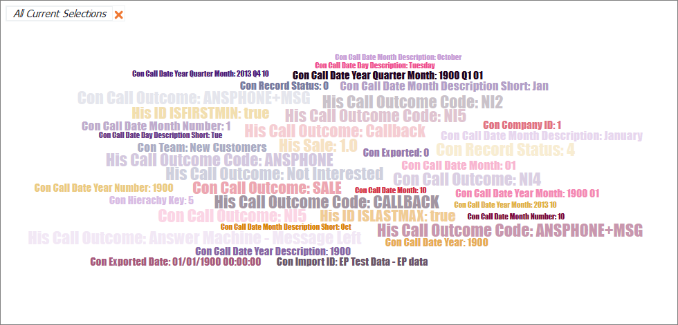
Displays fields with the highest probability represented by a larger font, allowing fast recognition of the most probable outcome.
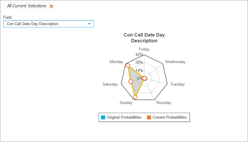
Displays fields and their original probabilities plotted against any manipulated probabilities. Use the Field drop-down list to display specific fields within the network for fast recognition of changed outcomes.
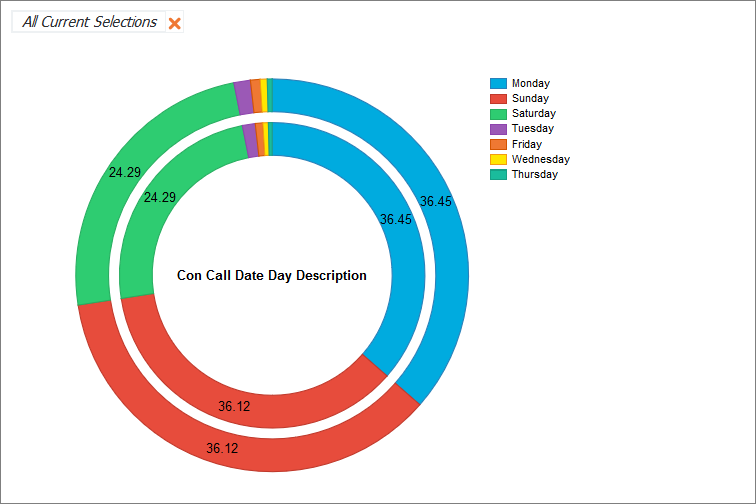
Displays a doughnut chart for each field that updates as probabilities are manipulated, showing a visual representation of percentages for presentational purposes.
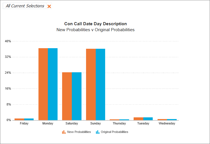
Displays the difference between original and manipulated probabilities for each field in a column chart that will update as probabilities are manipulated.
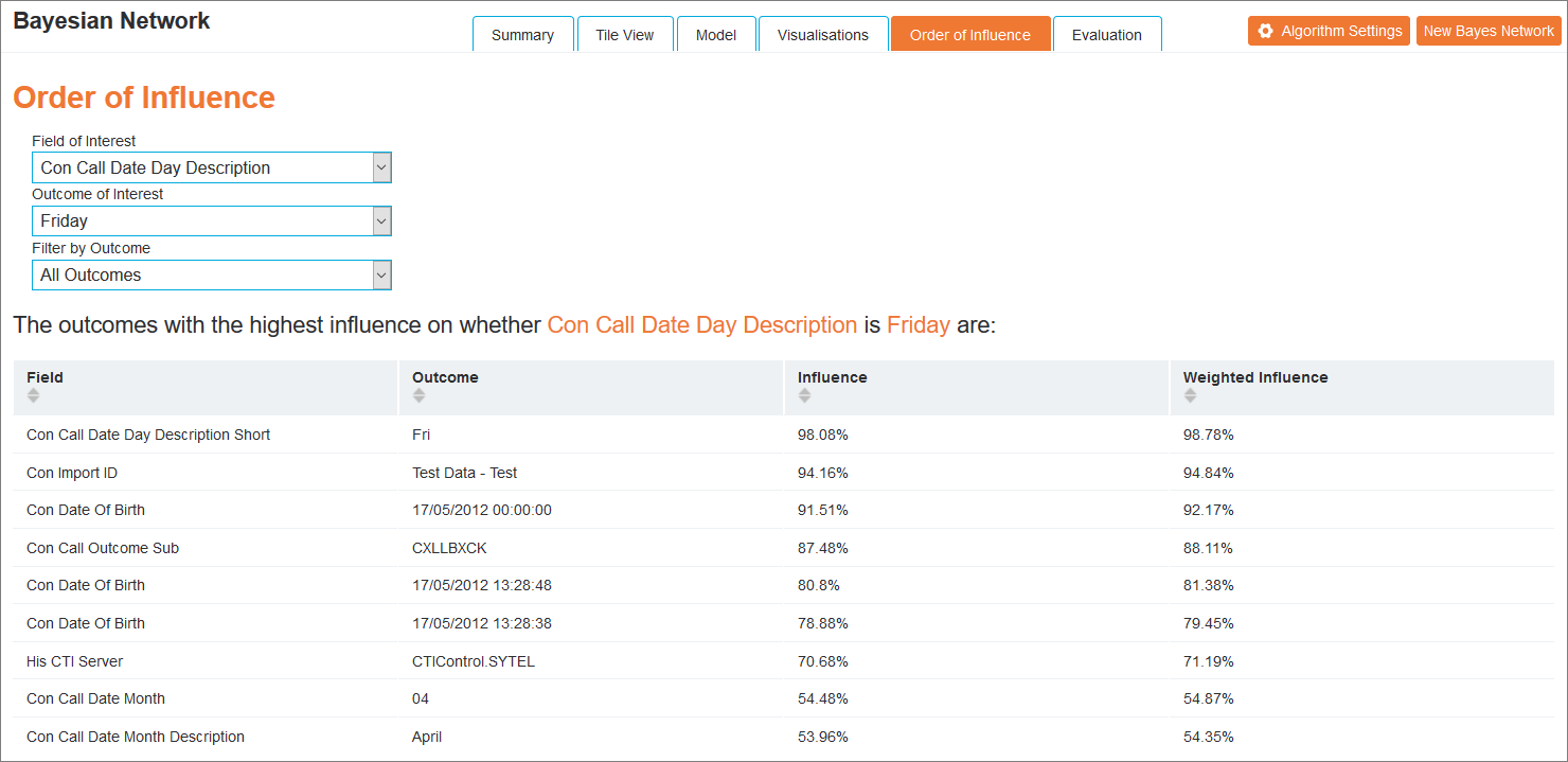
Using this view, it is possible to view the outcomes with the highest influence on a specific result. Each field is displayed with the Outcome, Influence and Weighted Influence.
The Weighted Influence is the current Influence divided by the total possible change when an outcome is selected. This gives a weighted score that reflects not only the influence, but the overall percentage change that is possible.
Choose a field from the Field of Interest drop-down list and select an outcome from the Outcome of Interest drop-down list. The Filter by Outcome drop-down list will constrain the results to those that match a specific outcome.
Using the default algorithm settings, 80% of the data is used to generate the network and the remaining 20% is used for testing the performance of the network. In this scenario, the Evaluation view will display the results of the analysis detailed below.
If the network has been generated from 100% of the data, there are two options for evaluation:
-
Cross validation first divides the dataset into five parts. Four of the pieces are used for training and the last piece is used for testing. This is repeated for all five pieces of the dataset and the results of the evaluation are averaged.
To run this evaluation, click Run Cross Validation. The results of the analysis will then be displayed.
Note: Running cross validation takes approximately five times longer to generate the network.
- Rerunning the Network with 80% of the data is also an option, using the remaining 20% for training and to test the model for accuracy. Click Rerun Network with 80/20 Split to generate the model with this analysis.
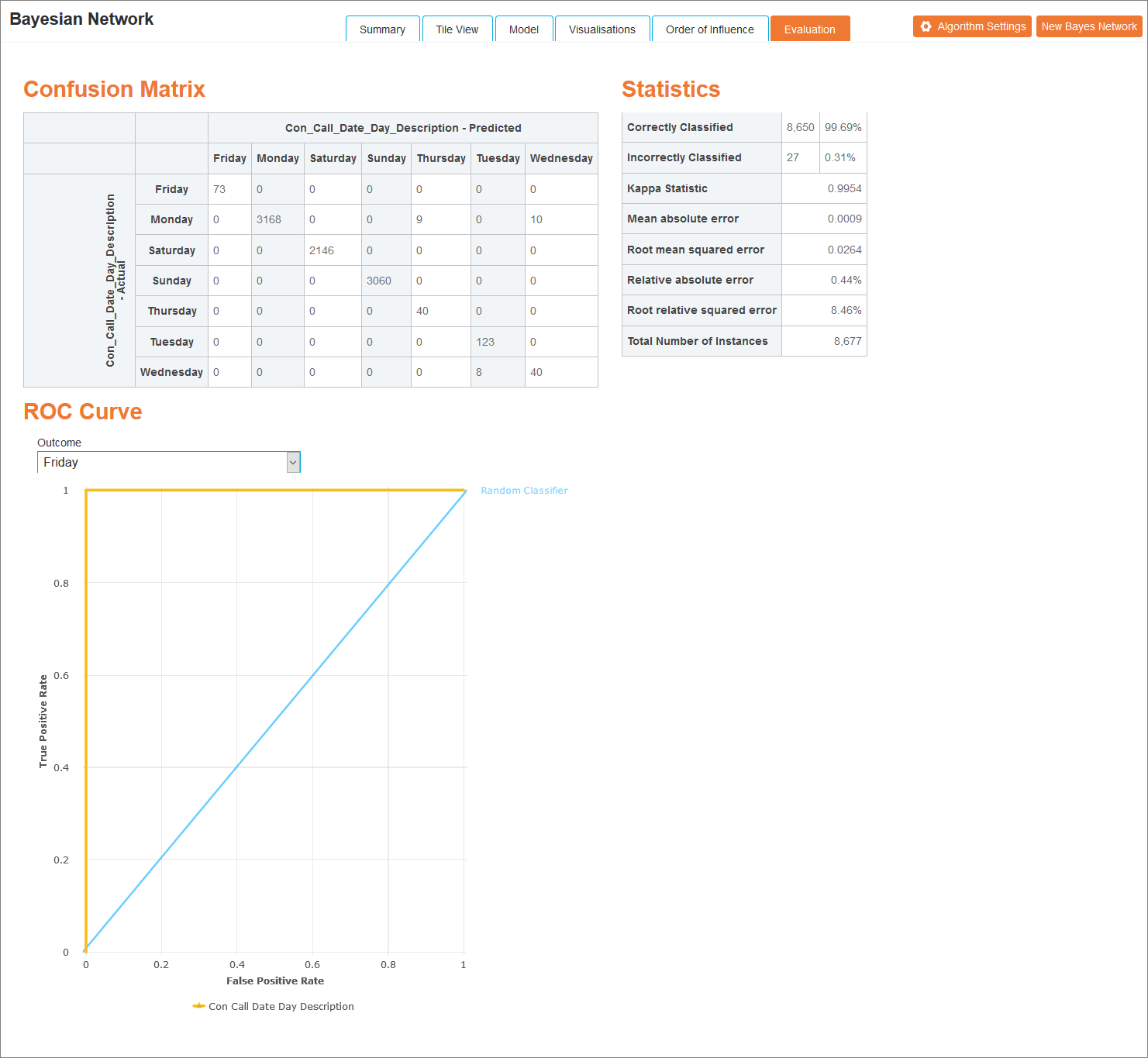
Once one of these options has been selected, statistics evaluating the classifier node are available.
For each row of data in the test set, the value of the classifier variable predicted by the network is compared with the actual value. The variables correctly classified will be in a diagonal line from the top left to the bottom right of the table.
The following analysis is performed on the network:
| Analysis | Description |
|---|---|
| Correctly Classified | The number of rows in the test set for which the classifier variable was correctly classified by the network. |
| Incorrectly Classified | The number of rows in the test set for which the classifier variable was classified incorrectly by the network. |
| Kappa Statistic |
Classification accuracy normalised by the imbalance of the classes in the data. An alternative to simple percentage agreement calculation that takes into account the possibility of the agreement occurring by chance. The closer the result is to 1, the more accurately the network has classified the variables. |
| Mean Absolute Error |
Measures how close forecasts or predictions are to the eventual outcomes regardless of direction. The closer the result is to 1, the less accurately the network has scored. A score of 0 indicates no errors. |
| Root Mean Squared Error |
Represents the same standard deviation of the differences between predicted values and observed values. The greater difference between the Root Mean Squared error and the Mean Absolute Error is the greater the variance in the individual errors in the sample. If two measures are equal, then all the errors are of the same magnitude. The closer the result is to 1, the less accurately the network has scored. A score of 0 indicates no errors. |
| Relative Absolute Error | Takes the total absolute error and normalises it by dividing by the total absolute error of the simple predictor that classifies variables randomly. |
| ROC Curve | Select a value from the Outcome drop-down list. The resulting ROC curve plots the true positive rate against the false positive rate for varying threshold values on the probability estimates. For example, a threshold value of 0.5 means that the predicted probability of ‘positive’ must be higher than 0.5 for the instance to be predicted as ‘positive’. This displays the model’s ability to predict the outcome compared to a random classifier. |